3.b. Colors
The goal of this analysis is to build a color palette of my haiku dataset, in the same vein as a 2017 PyCon talk titled Gothic Colors: Using Python to understand color in nineteenth century literature. This talk was the first exposure I can recall of the application of (hard) computer science to a (soft) natural science, and that made a lasting impression. The field of natural computing is eminently fascinating to me, and this conference talk was, in part, the inspiration behind my entire haiku generation project, going back even before trumperator, my first attempt at text generation. As an aside, after this project is good and finished, and I've settled into gainfully-employed life as a software engineer, I'd like to return to the generation of Trump tweets, using the same strategy as I've used here for haiku.
I'm getting carried away, however. Here, all I want to do, is parse the usage of color from the haiku in an intelligent manner—one that is aware that the word "rose" has three distinct meanings in the sentences
- "I picked a rose."
- "Her shoes were rose-colored."
- "He rose to meet me."
In the context of color parsing, it makes sense to treat the first two both as uses of the color "rose". In order to perform this parsing, we must part-of-speech tag the haiku corpus. Fortunately, doing so is not a new problem, so we use an out-of-the-box POS tagger.
import collections
import colorsys
import itertools

import matplotlib.pyplot as plt
import nltk
import numpy as np
import pandas as pd
import seaborn as sns
import webcolors
from IPython.display import Image

import haikulib.eda.colors
from haikulib import data, nlp, utils
sns.set(style="whitegrid")
The Naive Approach
It's often useful to implement a simpler version of a feature before implementing the full functionality. So before performing POS-tagging and more intelligent color identification, we simply look for color names in the corpus. We do so by looking for any n-grams that are in our master list of color names. We use 1, 2, and 3-grams.
df = data.get_df()
corpus = []

for haiku in df["haiku"]:
    corpus.append(" ".join(haiku.split("/")))

color_names = {r["color"]: r["hex"] for _, r in haikulib.eda.colors.get_colors().iterrows()}
naive_colors = collections.Counter()
for haiku in corpus:
    # Update the color counts for this haiku.
    naive_colors.update(nlp.count_tokens_from(haiku, color_names, ngrams=[1, 2, 3]))
For ease of use in visualization, I build a data frame of the color occurrences.
naive_color_counts = pd.DataFrame({
        "color": list(naive_colors.keys()),
        "count": list(naive_colors.values()),
        "hex": [color_names[c] for c in naive_colors],
    })
total_color_count = sum(row["count"] for index, row in naive_color_counts.iterrows())

print(f"There are {total_color_count} occurences of color in the corpus")
print(f"There are {len(naive_color_counts)} unique colors")
naive_color_counts.head(10)| # | color | count | hex |
|---|---|---|---|
| 0 | green | 415 | #3aa655 |
| 1 | snow | 1981 | #fffafa |
| 2 | dusk | 482 | #4e5481 |
| 3 | sea | 679 | #3c9992 |
| 4 | watermelon | 27 | #fd4659 |
| 5 | sky | 1232 | #82cafc |
| 6 | stone | 275 | #ada587 |
| 7 | jasmine | 66 | #f8de7e |
| 8 | sand | 300 | #c2b280 |
| 9 | rust | 27 | #b7410e |
Color Parsing with Part-Of-Speech Tagging
These analyses were originally done in Jupyter Notebooks, and converted to HTML (by hand, because I'm not good enough with pandoc or nbconvert to match my website's custom CSS and boostrap classes).
Rather than implement the color parsing as a part of the notebook, and then copy paste the
implementation to do analysis later, the color parsing was done in the
haikulib.eda module. But for the sake of self-contained notebooks, I wanted a way to
show the source of an arbitrary function so I'm not copy-pasting out-of-sync versions of function
around. So I wrote a small introspective helper function to grab the source code of a function and
render it in syntax-highlighted HTML in the Jupyter notebook.
# Use display_source() to display its own source. This feels dirty.
utils.display_source("haikulib.utils", "display_source")
def display_source(module: str, function: str) -> IPython.display.Code:
"""Display the source of the provided function in a notebook.
:param module: The module containing function. Must be importable.
:param function: The function whose source we wish to display.
"""
__module = importlib.import_module(module)
__methods = dict(inspect.getmembers(__module, inspect.isfunction))
def _jupyterlab_repr_html_(self):
from pygments import highlight
from pygments.formatters import HtmlFormatter
fmt = HtmlFormatter()
style = "<style>{}\n{}</style>".format(
fmt.get_style_defs(".output_html"), fmt.get_style_defs(".jp-RenderedHTML")
)
return style + highlight(self.data, self._get_lexer(), fmt)
# Replace the _repr_html_() method with our own that also adds the `jp-RenderedHTML` class
# to fix https://github.com/jupyterlab/jupyterlab/issues/6376.
# Mmmm. Slimy.
IPython.display.Code._repr_html_ = _jupyterlab_repr_html_
return IPython.display.Code(data=inspect.getsource(__methods[function]), language="python3")However, I haven't figured out a good (minimal) way to style individual notebook cells, so I'll break from the real notebook and continue as if the color parsing functions are defined in the notebook itself.
We can determine if a word is a color simply by checking if it is contained in our color master list, and by checking if it is an adjective or a noun.
def __get_colors() -> pd.DataFrame:
    """Get a DataFrame of color -> HTML colors.
    Note that this CSV file uses hex RGB color codes for many of the colors, but falls back to using
    HTML named colors for colors without an RGB value.
    The colors with RGB values came from https://xkcd.com/color/rgb/ while the colors with the named
    values came from
    https://medium.com/@eleanorstrib/python-nltk-and-the-digital-humanities-finding-patterns-in-gothic-literature-aca84639ceeb
    """
    return pd.read_csv(data.get_data_dir() / "colors.csv", index_col=0)

def __get_colors_dict() -> dict:
    """Get a dictionary of color -> HTML color mappings."""
    df = __get_colors()
    return {row["color"]: row["hex"] for index, row in df.iterrows()}

COLORS = __get_colors_dict()
COLOR_POS_TAGS = frozenset({"JJ", "NN"})

def is_color(tagged_word: Tuple[str, str]) -> bool:
    """Determine if the given word is a color based on its part-of-speech.
    :param tagged_word: A word that's been tagged with nltk.pos_tag()
    """
    word, pos = tagged_word
    return pos in COLOR_POS_TAGS and word in COLORS
However, this requires on each work in the corpus being tagged with its part of speech. This too is simple
def pos_tag(text: str) -> Iterable[Tuple[str, str]]:
    """Part-of-speech tag the given text.
    """
    return nltk.pos_tag([w for w in text.split() if w not in {"/"}])
Now we can quite simply find the colors in a particular haiku as follows.
# A made-up haiku for testing purposes.
haiku = "dark blue lines / in a light olive green sea salt / dreams"
haiku_colors = [
    tagged_word[0]
    for tagged_word in nlp.pos_tag(haiku)
    if haikulib.eda.colors.is_color(tagged_word)
]
print(haiku_colors)
this gives
['dark', 'blue', 'olive', 'green', 'sea']But wait a minute! What about the color "dark blue", or "olive green"? In order to find multi-word colors, we need to parse and test n-grams from the haiku. Unfortunately it was quite late when I implemented this, so I was frustrated, and made it "just work" with no care for doing it right. It shows.
def find_colors(text: Iterable[Tuple[str, str]]) -> List[str]:
    """Return an unordered list of colors from the given POS-tagged text.

    Check for 1, 2, and 3-gram colors like "dark blue".

    Attempt to make the 1, 2, 3-grams exclusive so that a text containing "light olive green"
    (#a4be5c) will return just
        ["light olive green"]
    instead of
        ["light", "olive", "green", "olive green", "light olive green"]

    :param text: The POS-tagged text to search for colors.
    :return: A list of colors appearing in the provided text.
    """
    colors = []

    # Pad the right of any text that is too short to prevent a nasty crash.
    ngrams = nltk.ngrams(text, n=3, pad_right=True, right_pad_symbol=("?", "??"))
    for ngram in ngrams:
        word = " ".join(w[0] for w in ngram)
        # Check the 3-gram
        if word in COLORS:
            colors.append(word)
            # Skip over the rest of this ngram.
            next(ngrams)
            next(ngrams)
        # If the 3-gram wasn't a color, check the 2-gram.
        else:
            word = " ".join(w[0] for w in ngram[:2])
            if word in COLORS:
                colors.append(word)
                # Skip over the rest of this ngram.
                next(ngrams)
            # If the 2-gram wasn't a color, check the 1-gram, using the tagged part-of-speech.
            elif is_color(ngram[0]):
                colors.append(ngram[0][0])

    try:
        # Check the last 2-gram and the last two 1-grams by hand (skipped by loop)
        if ngram[1:] in COLORS:
            word = " ".join(w[0] for w in ngram[1:])
            colors.append(word)
        else:
            if is_color(ngram[-2]):
                colors.append(ngram[-2][0])
            if is_color(ngram[-1]):
                colors.append(ngram[-1][0])
    except UnboundLocalError:
        # As with life, problems are best left ignored.
        pass

    return colors
Notice that we only use is_color() for checking if 1-grams are colors. 2-grams and 3-grams
use a simple containment check against the color master list. Further, notice that there is
soul-crushing logic used to parse the colors ["light olive green", "sea"] from the string
"light olive green sea" instead of the colors
["olive", "green", "sea", "olive green", "light olive green"].
It even works on our test haiku that we defined.
find_colors(nlp.pos_tag(haiku))gives us ['dark blue', 'light olive green', 'sea'].
Then we parse the colors from the haiku during the repository data initialization step so that they are
stored in the data/haiku.csv file. If we record the color usage for each haiku
individually, that enables spatial exploration of the colors.
df = data.get_df()
df.tail(6)| # |
haiku | colors |
lines | syllables | total_syllables |
|---|---|---|---|---|---|
| 55357 | shadows a window ledge / just big enough to hold / two doves | [] | 3 | (7, 6, 3) | 16 |
| 55358 | sparks / in the heat of blue / dragonflies | [blue] | 3 | (1, 5, 3) | 9 |
| 55359 | half moon / only broken crackers / in the tin | [] | 3 | (2, 6, 3) | 11 |
| 55360 | revision notes / brushing sand / into the gaps | [sand] | 3 | (5, 3, 4) | 12 |
| 55361 | the first dusk of may / it's suddenly there / a pale orange poppy | [dusk, pale orange] | 3 | (5, 6, 7) | 18 |
| 55362 | dandelions / two drinkers unzip / by the path | [] | 3 | (3, 5, 3) | 11 |
| 55363 | scrunched up clouds / a blue plastic bag / in the nettles | [blue] | 3 | (4, 5, 4) | 13 |
| 55364 | early spring / one morning the clang of / scaffolding poles | [] | 3 | (3, 7, 5) | 15 |
| 55365 | platform 9 / through the glass roof the shapes / of swooping gulls | [glass] | 3 | (3, 7, 4) | 14 |
| 55366 | sneaking out / thru' the bathroom window / steam meets fog | [] | 3 | (3, 6, 3) | 12 |
As above, we also produce a data frame containing the corpus color counts and HTML color codes.
pos_tagging_color_counts = haikulib.eda.colors.get_colors()

total_color_count = pos_tagging_color_counts["count"].sum()
used_color_count = pos_tagging_color_counts["count"].astype(bool).sum(axis=0)

print(f"There are {total_color_count} occurences of color in the corpus")
print(f"There are {used_color_count} unique colors")

pos_tagging_color_counts[["color", "count", "hex"]].head(10)| # | color |
count |
hex |
|---|---|---|---|
| 0 | cloudy blue | 0 | #acc2d9 |
| 1 | dark pastel green | 0 | #03c03c |
| 2 | dust | 207 | #b2996e |
| 3 | electric lime | 0 | #ccff00 |
| 4 | fresh green | 0 | #69d84f |
| 5 | light eggplant | 0 | #894585 |
| 6 | nasty green | 0 | #70b23f |
| 7 | really light blue | 0 | #d4ffff |
| 8 | tea | 246 | #65ab7c |
| 9 | warm purple | 0 | #952e8f |
Compare the POS-tagging results with those from the naive approach, summarized again below. Notice that we pruned over twenty color names from the corpus, and pruned over three thousand occurrences of colors.
total_color_count = naive_color_counts["count"].sum()

print(f"There are {total_color_count} occurences of color in the corpus")
print(f"There are {len(naive_color_counts)} unique colors")

naive_color_counts.head(10)| # | color | count | hex |
|---|---|---|---|
| 0 | green | 415 | #3aa655 |
| 1 | snow | 1981 | #fffafa |
| 2 | dusk | 482 | #4e5481 |
| 3 | sea | 679 | #3c9992 |
| 4 | watermelon | 27 | #fd4659 |
| 5 | sky | 1232 | #82cafc |
| 6 | stone | 275 | #ada587 |
| 7 | jasmine | 66 | #f8de7e |
| 8 | sand | 300 | #c2b280 |
| 9 | rust | 27 | #b7410e |
Color Palette Visualization
Now that we've extracted the uses of color from the corpus, there are a number of techniques we can use to visualize that data. We will use the following methods:
- Word cloud
- Histogram
- Pie Chart
- Spectrum
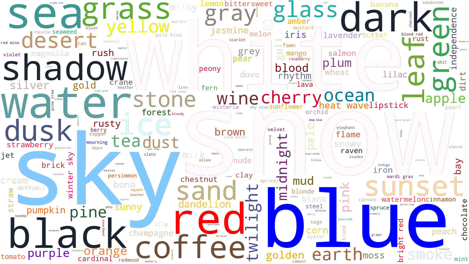
Word Cloud
See Word Clouds for a discussion of how to generate the word clouds for the haiku vocabulary in the general case, as well as restricted to flora, fauna, and colors. The color word cloud is reproduced below.
Histogram
The color histogram, sorted by frequency, is show below.
colors = haikulib.eda.colors.get_colors()
colors.sort_values(by=["hsv", "count"], ascending=False, inplace=True)
used_colors = colors.loc[colors["count"] != 0].copy()
used_colors.sort_values(by="count", ascending=False, inplace=True)

_ = plt.bar(
    range(len(used_colors)),
    used_colors["count"],
    color=used_colors["rgb"],
    width=1,
    linewidth=0,
    log=True,
)
plt.show()
However, there are other ways we might display the same information.
used_colors.sort_values(by="hsv", ascending=False, inplace=True)
_ = plt.bar(
    range(len(used_colors)),
    used_colors["count"],
    color=used_colors["rgb"],
    width=1,
    linewidth=0,
    log=True,
)
plt.show()
background = plt.bar(
    range(len(colors)),
    height=12 ** 3,
    width=1,
    linewidth=0,
    color=colors["rgb"],
    log=True,
    alpha=0.8,
)
foreground = plt.bar(
    range(len(colors)),
    height=colors["count"],
    width=3,
    linewidth=0,
    color="black",
    log=True,
)
plt.show()
We have several options for using a polar histogram:
- Sort the colors radially, by their hue or their frequency
- Use fixed or proportional radii
- Use fixed or proportional wedge widths
- Use a fixed or proportional division of [0, 2pi] for the wedges angular locations
def pairwise_difference(seq):
    for l, r in utils.pairwise(seq):
        yield r - l
    # Loop back around to the front.
    yield 2 * np.pi - seq[-1]


def accumulate(seq):
    _sum = 0
    for s in seq:
        yield _sum
        _sum += s
First, we'll sort the colors by their frequency and display them radially.
used_colors.sort_values(by="count", ascending=False, inplace=True)

ax = plt.subplot(111, projection="polar")

thetas = 2 * np.pi * used_colors["count"] / used_colors["count"].sum()
thetas = np.array(list(accumulate(thetas)))
widths = np.array(list(pairwise_difference(thetas)))
radii = np.log(used_colors["count"])

_ = ax.bar(
    x=thetas,
    height=radii,
    width=widths,
    color=used_colors["rgb"],
    linewidth=0,
    align="edge",
)
plt.show()
ax = plt.subplot(111, projection="polar")

_ = ax.bar(
    x=thetas,
    # Plot the same information with a fixed height.
    height=1,
    width=widths,
    color=used_colors["rgb"],
    linewidth=0,
    align="edge",
)
plt.show()
I wanted to get a sense of the color palette in general, so let's try to sort the colors by hue. Unfortunately, this is a hard problem in general, because colors are three-dimensional, and we are attempting to sort them in a single dimension! There are techniques that utilize Hilbert curves to sort colors in two dimensions, but for now sorting by hue is sufficient.
ax = plt.subplot(111, projection="polar")

thetas = np.linspace(0, 2 * np.pi, len(used_colors), endpoint=False)
widths = 4 * np.pi / len(used_colors)
radii = np.log(used_colors["count"])

_ = ax.bar(
    x=thetas,
    height=radii,
    width=widths,
    color=used_colors["rgb"],
    linewidth=0,
    align="edge",
)
plt.show()
ax = plt.subplot(111, projection="polar")

thetas = 2 * np.pi * used_colors["count"] / used_colors["count"].sum()
thetas = np.array(list(accumulate(thetas)))
widths = np.array(list(pairwise_difference(thetas)))
radii = np.log(used_colors["count"])

_ = ax.bar(
    x=thetas,
    height=1,
    width=widths,
    color=used_colors["rgb"],
    linewidth=0,
    align="edge",
)
plt.show()
ax = plt.subplot(111, projection="polar")

_ = ax.bar(
    x=thetas,
    height=radii,
    width=widths,
    color=used_colors["rgb"],
    linewidth=0,
    align="edge",
)
plt.show()
I have no real conclusion, other than people who know how to do real color visualization are a lot smarter than I am. I thought this was cool, but ultimately I wasn't able to make any conclusions.