1.c. Neural Networks

Much of the future discussion on neural network language models will require at least an intuitive understanding of neural networks. This section aims to provide enough background and vocabulary to facilitate discussion of neural networks as a concept without becoming bogged down in a nontrivial amount of detail.

There are many other excellent introductions to neural networks that provide much more detail such as for a general mathematical treatment, or for a treatment specific to processing natural language.

A Biological Metaphor

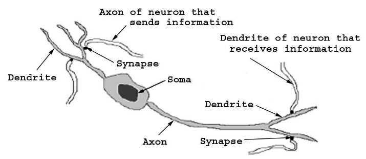
If our intent is to produce intelligent, sophisticated statistical models, it is useful to motivate our model with the biological metaphor of a single neuron. Of course, our intent is not to emulate, nor is it to simulate a collection of biological neurons. We simply wish to motivate a mathematical discussion of a statistical model that has proved useful in data analysis, modeling, and prediction. In this spirit, we note that it is well beyond the scope of this paper to provide a biologically correct description of the hugely complex field of neuroscience. In fact, it would be reasonable to present neural networks devoid of any biological motivation simply as a mathematical model that has proven to be useful.

The figure above shows a "typical" neuron (of course there is no such thing) with various labeled components. In the most general sense, a neuron takes electrical stimulation through its dendrites, processes the received information, and under the right conditions emits a signal through its axon to the dendrites of an adjacent neuron . Somehow, through an organization of many such neurons, intelligent behavior emerges .

An Artificial Neuron

Even such a grossly simplified treatment of a neuron provides motivation for the artificial neuron shown below

The artificial neuron, called a unit, takes a fixed number of inputs \(x_0, \dots, x_n\), multiplies each with its corresponding weight, and adds the weighted inputs together before piping the result through the activation function \(f\). Note that if the inputs are treated as a column vector \(\vec x\), and the weights as a vector \(\vec w\), the output is the result of the operation \(y = f(\vec w \cdot \vec x)\).

Often it is useful to add a bias term \(b\)

\[y = f(\vec w \cdot \vec x + b)\]

by adding a fixed unitary input to the neuron. This allows us to treat the bias term exactly like one of the weights when assembling multiple such units together to form a network.

Assembling Collections of Neurons into Networks

Presumably then, the intelligence of a neural network has something to do with how the units are assembled together, and with the magical weight values associated with each unit. Unlike the chaotic and organic layout in the human body, we assemble the artificial neurons into sequential layers, and connect the outputs of the previous layer to the inputs of the next.

When we treat the cells as a vertical layer, we get

\[\vec y = f(W^T \vec x + \vec b)\]

where each of the weight vectors \(\vec w\) for each cell is arranged into the matrix \(W\), and each of the \(y\)-values are concatenated to form \(\vec y\). Common choices for the activation function \(f\) are the hyperbolic tangent, sigmoid, rectified linear unit, and softmax functions. Note that the use of \(f\) in the above equation assumes that the same activation function is used for every unit in the layer.

Due to the large amount of homogeneity in the units for each layer, we almost never draw schematic diagrams of a network's architecture showing the individual units. Instead, we treat the layer of units as the basic abstraction as in the figure below

The dimension of each layer is shown at the top of each layer, and the activation function of the non-input layers is indicated below each layer. The underlying mathematical operation that this architecture defines is

\[\vec y = \softmax\left(W_2^T \tanh(W_1^T \vec x + \vec{b_1}) + \vec{b_2}\right)\]

where \(\vec{b_1}\) and \(\vec{b_2}\) are the implicit bias vectors, and \(W_1\) and \(W_2\) are the weight matrices for the \(\tanh\) and \(\softmax\) layers respectively.

Here, the softmax activation function

\[\softmax(\vec x) = \frac{\exp\left(\vec x\right)}{\sum\exp\left(\vec x\right)}\]

is applied element-wise to the vector \(\vec x\), and produces the vector \(\vec y\) which can be treated as a probability distribution over \(n\) values. That is, the vector \(y\) sums to 1. The softmax activation function is often used in neural networks whose output is to be treated as a probability, and will be used extensively in language modeling.