3.e. Zipf's Law

This was the first exploratory data analysis I did on the haiku corpus, and is also the least illuminating. However, it provided an opportunity to get started digging in to the dataset, and inspired some of the other explorations that were useful.

Zipf's law states that the frequencies of words from a natural language corpus are inversely proportional to their rank in a frequency table. That is, a plot of their rank vs frequency on a log-log scale will be roughly linear. Consider the following entirely contrived example. The first word is twice as frequent as the second, and three times as frequent as the third.


rank	value	occurrences
1	word 1	21
2	word 2	10
3	word 3	7

If we plot the rank vs frequency on a log-log plot, we get the following

import operator
from collections import Counter
from urllib.request import urlopen

import matplotlib.pyplot as plt
import nltk
import numpy as np
import pandas as pd
import seaborn as sns

from haikulib import data, nlp, utils
sns.set(style="whitegrid")

ranks = np.array([1, 2, 3])
frequencies = np.array([21, 10, 7])

plt.plot(np.log(ranks), np.log(frequencies))
plt.plot(np.log(ranks), np.log(frequencies), ".")

plt.xlabel("$\log(rank)$")
plt.ylabel("$\log(freq)$")
plt.show()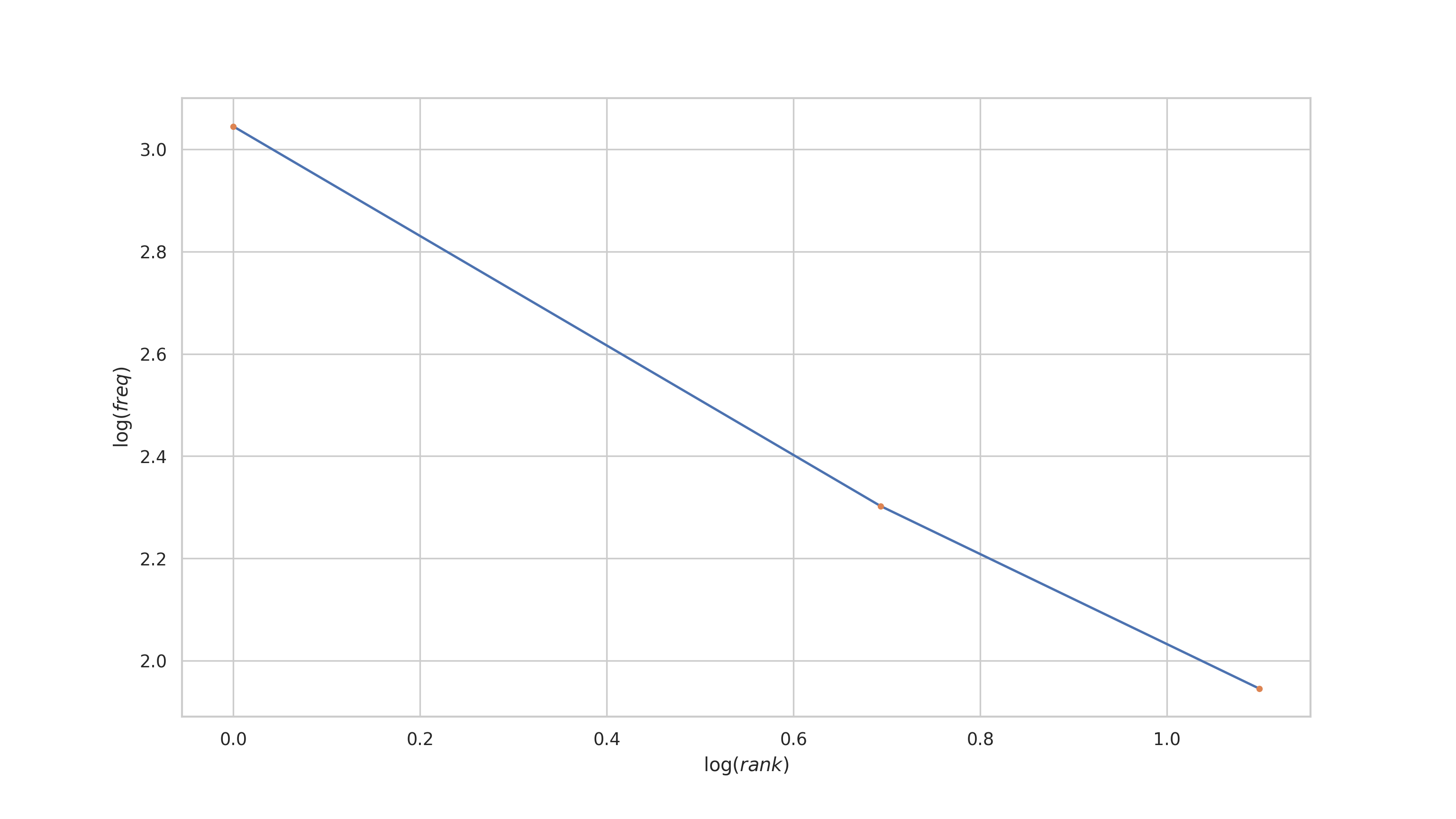

A contrived log-log plot of rank vs frequency — A log-log plot of the rank vs frequency of the contrived data

The supposition was that haiku are a compressed form of expression, so perhaps Zipf's law might not hold. That means that we should examine how Zipf's law holds up for a non-haiku corpus to build a baseline before we procede to haiku. I'm a sucker for the dark, cynical, misanthropic Ambrose Bierce, so let's download his collected works from Project Gutenberg and examine how the look with respect to Zipf's law.

One of the ways to represent a natural language corpus, is with what's called a bag-of-words representation, where all of the individual words in the corpus have been tossed into a bag, without their surrounding context, much like a bag of Scrabble tiles. This is a natural representation for the present work, as examining individual word frequencies does not require surrounding context.

The frequency table is just another view of the bag-of-words. It contains no new information, it's just formatted a little differently to make mathematical analysis a bit easier.

def get_freq_table(bag):
    """Get a frequency table representation of the given bag-of-words representation."""
    assert isinstance(bag, Counter)
    words, frequencies = zip(
        *sorted(bag.items(), key=operator.itemgetter(1), reverse=True)
    )
    words = np.array(words)
    frequencies = np.array(frequencies)
    ranks = np.arange(1, len(words) + 1)

    freq_table = pd.DataFrame({"rank": ranks, "word": words, "frequency": frequencies})
    return freq_table

part1 = 'https://www.gutenberg.org/cache/epub/13541/pg13541.txt'
part2 = 'https://www.gutenberg.org/cache/epub/13334/pg13334.txt'

part1 = urlopen(part1).read().decode("utf-8")
part2 = urlopen(part2).read().decode("utf-8")

corpus = " ".join(part1.split()) + " ".join(part2.split())
tokens = [nlp.preprocess(t) for t in corpus.split()]
bag = Counter(tokens)
freq_table_bierce = get_freq_table(bag)
freq_table_bierce.head()


rank	word	frequency
1	the	11255
2	of	6628
3	and	4648
4	a	4056
5	to	3943

plt.plot(
    np.log(freq_table_bierce["rank"]),
    np.log(freq_table_bierce["frequency"]),
    ".",
    markersize=3,
)

plt.xlabel("$\log(rank)$")
plt.ylabel("$\log(freq)$")
plt.show()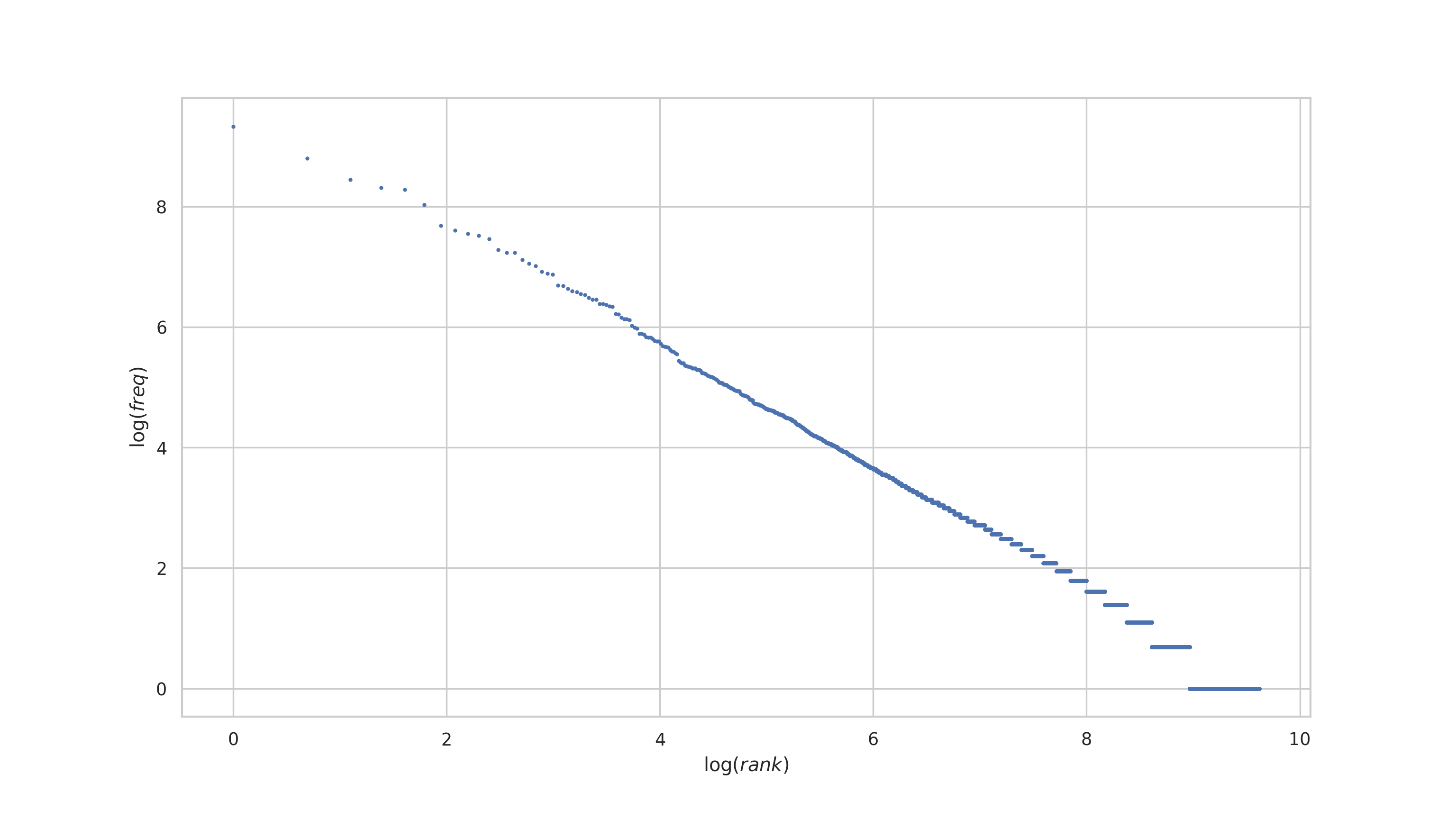

A log-log plot of the rank vs frequency for Ambrose Bierce's works — A log-log plot of rank vs frequency for Ambrose Bierce's works

We see that Zipf's law does indeed hold for Ambrose Bierce's work. The log-log plot is roughly linear!

Now, consider what happens when we remove the stopwords (fillers) from the corpus. These are words like "a", "an", "the", "to", etc. What might happen to the log-log plot?

for stopword in nlp.STOPWORDS:
    if stopword in bag:
        del bag[stopword]

stop_table_bierce = get_freq_table(bag)

plt.plot(
    np.log(freq_table_bierce["rank"]),
    np.log(freq_table_bierce["frequency"]),
    ".",
    markersize=3,
    label="bierce with stopwords",
)
plt.plot(
    np.log(stop_table_bierce["rank"]),
    np.log(stop_table_bierce["frequency"]),
    ".",
    markersize=3,
    label="bierce without stopwords",
)

plt.xlabel("$\log(rank)$")
plt.ylabel("$\log(freq)$")
plt.legend()
plt.show()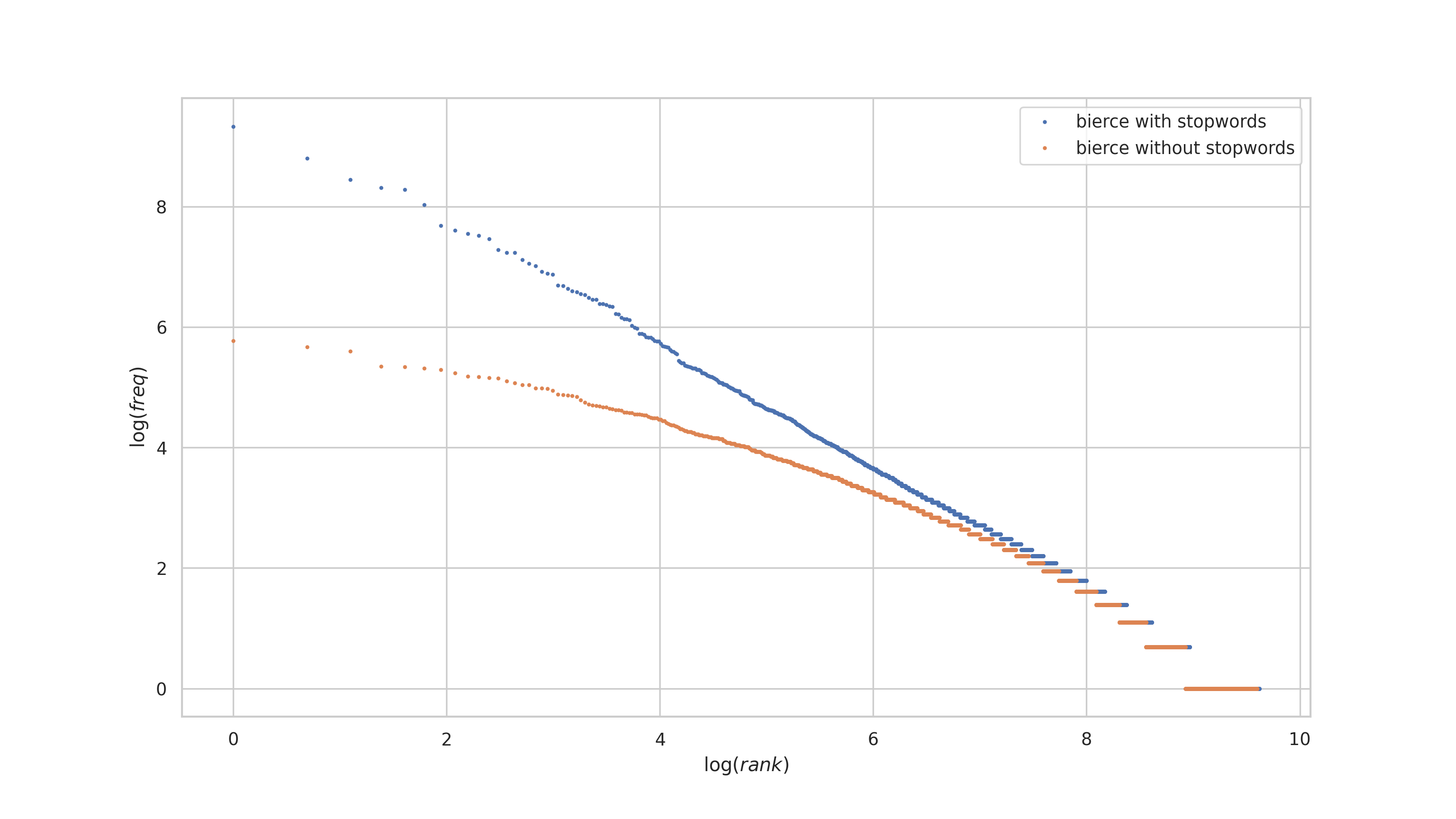

A log-log plot of rank vs frequency for Ambrose Bierce's works without stopwords

Notice that the log-log plot has a slight curve in it, when stopwords are removed! So what might we expect from haiku, a condensed form of natural language expression, with limitations on the words one can use?

bag = data.get_bag_of(kind="words", add_tags=False)
del bag["/"]
freq_table = get_freq_table(bag)
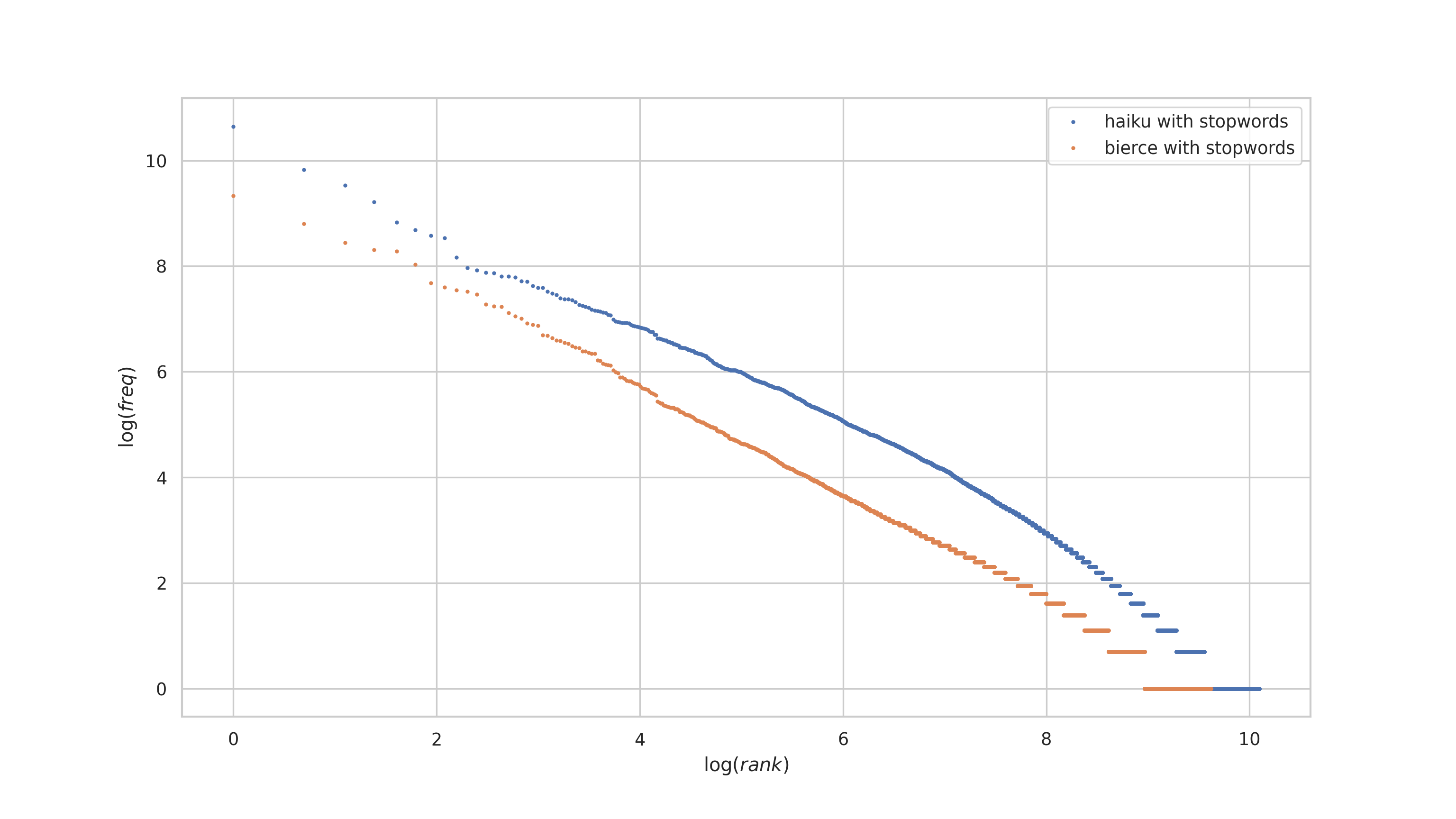
freq_table.head()

Looking at the top few words in the frequency table for the haiku bag-of-words, we see mostly the same most-frequent words as we did for Bierce's works. This isn't surprising, so we'll do as we did above, plot the ranks vs frequencies for the haiku corpus with that of Bierce's works, and compare.


rank	word	frequency
1	the	41980
2	a	18511
3	of	13732
4	in	10090
5	my	6855

plt.plot(
    np.log(freq_table["rank"]),
    np.log(freq_table["frequency"]),
    ".",
    markersize=3,
    label="haiku with stopwords",
)
plt.plot(
    np.log(freq_table_bierce["rank"]),
    np.log(freq_table_bierce["frequency"]),
    ".",
    markersize=3,
    label="bierce with stopwords",
)

plt.xlabel("$\log(rank)$")
plt.ylabel("$\log(freq)$")
plt.legend()
plt.show()

There are two things to notice:

The plots are offset from each other. This is expected, because the haiku corpus is larger than Bierce's (at least what I downloaded from Project Gutenberg).
The haiku plot is slightly curved!

A log-log plot of rank vs frequency for Bierce's works and the haiku corpus

Now for illustrative purposes, let's grab a few of the top most frequent words and annotate the plot with them.

def get_indices(df, column, values):
    """Gets the indices of values from the given column of the given dataframe."""
    indices = []
    for value in values:
        indices += df[column][df[column] == value].index.tolist()
    return indices

indices = get_indices(freq_table, "word", ["the", "a", "of", "to", "i", "her", "his"])
interesting = freq_table.loc[indices]

What comes next is unfortunate, but I'm not sure how to do it otherwise without a lot of extra work.

plt.plot(np.log(freq_table["rank"]), np.log(freq_table["frequency"]), ".", markersize=3)

# This should be a crime.
x_adjust = np.array([0.1, -0.6, 0.15, -0.6, 0.2, -0.6, 0.0])
y_adjust = np.array([1.0, -1.2, 1.0, -1.3, 1.0, -1.3, 1.0])

for word, freq, rank, xa, ya in zip(
    interesting["word"],
    interesting["frequency"],
    interesting["rank"],
    x_adjust,
    y_adjust,
):
    plt.annotate(
        word,
        xy=(np.log(rank), np.log(freq) + ya / 20),
        xytext=(np.log(rank) + xa, np.log(freq) + ya),
        size=9,
        arrowprops={"arrowstyle": "-", "color": "k"},
    )

plt.xlabel("$\log(rank)$")
plt.ylabel("$\log(freq)$")
plt.ylim((-0.5, 11.9))
plt.show()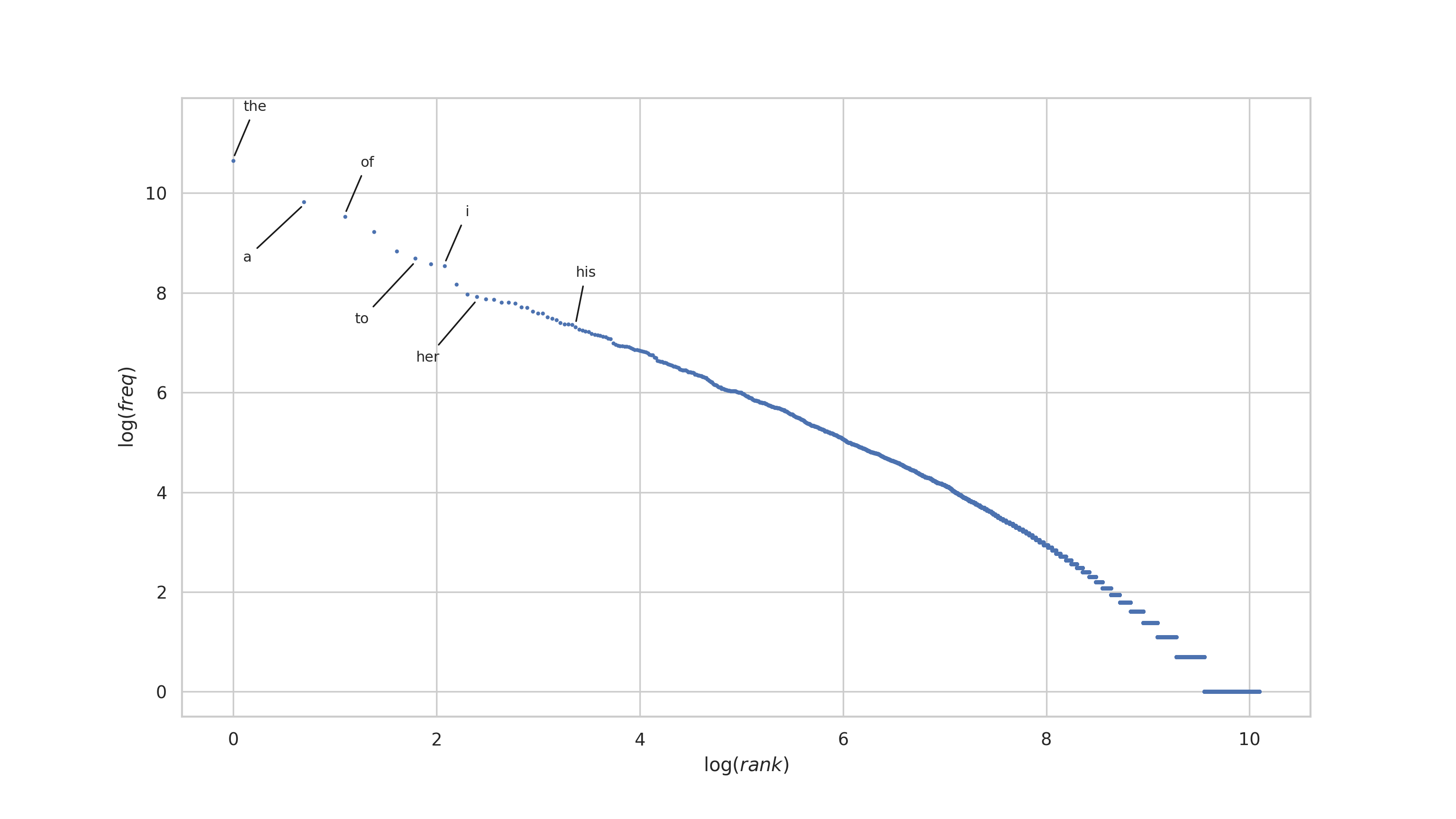

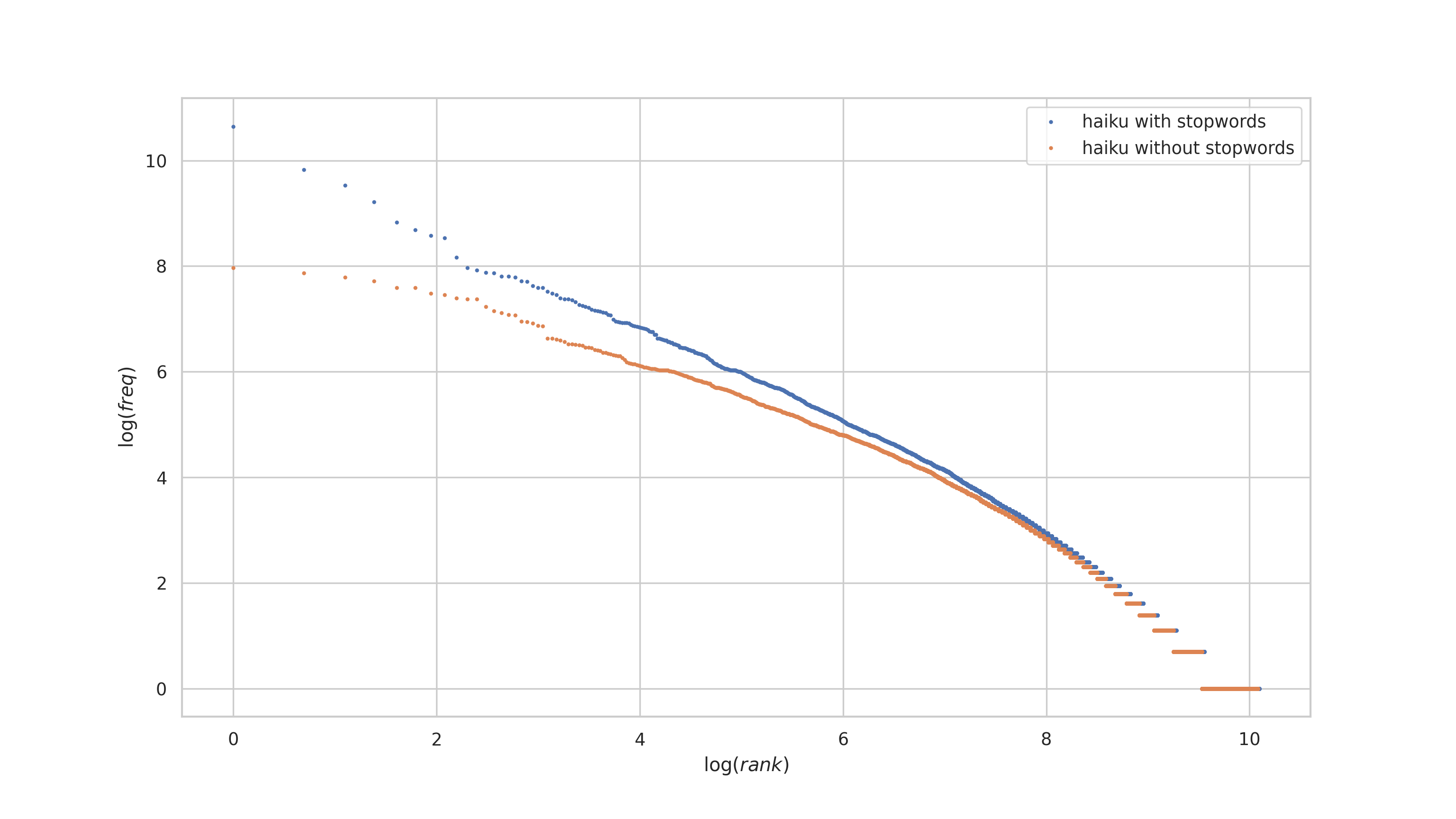
The haiku log-log rank vs frequency plot annotated with a few of the most frequent words

We proceed with removing stopwords from the haiku corpus.

for stopword in nlp.STOPWORDS:
    if stopword in bag:
        del bag[stopword]

stop_table = get_freq_table(bag)

plt.plot(
    np.log(freq_table["rank"]),
    np.log(freq_table["frequency"]),
    ".",
    markersize=3,
    label="haiku with stopwords",
)
plt.plot(
    np.log(stop_table["rank"]),
    np.log(stop_table["frequency"]),
    ".",
    markersize=3,
    label="haiku without stopwords",
)

plt.xlabel("$\log(rank)$")
plt.ylabel("$\log(freq)$")
plt.legend()
plt.show()

The result is similar to that of Bierce's works, but the difference between the plot for the haiku corpus with and without stopwords is much less pronounced. I interpret this as indicating that haiku are a compressed form of expression, but not as compressed as Bierce's written works without stopwords. Haiku become even more compressed when stopwords are removed, but the compression factor is not as severe as it is with Bierce's works.

The haiku log-log rank vs frequency plot with and without stopwords

We proceed building the annotated log-log plot for the haiku without stopwords as well.

stop_table.head(15)


rank	word	frequency
1	moon	2883
2	rain	2603
3	day	2405
4	night	2239
5	snow	1981
6	winter	1975
7	morning	1778
8	summer	1726
9	spring	1628
10	old	1590
11	wind	1589
12	autumn	1377
13	dog	1274
14	sky	1232
15	new	1189

indices = get_indices(
    stop_table,
    "word",
    ["moon", "rain", "day", "night", "snow", "winter", "summer", "spring", "autumn"],
)

interesting = stop_table.loc[indices]

plt.plot(np.log(stop_table["rank"]), np.log(stop_table["frequency"]), ".", markersize=3)

# This should also be a crime.
x_adjust = np.array([-0.35, -0.9, -0.23, -0.9, -0.1, -0.7, 0.3, -0.7, 0.4])
y_adjust = np.array([1.0, -1.0, 1.1, -1.1, 1.1, -1.4, 1.0, -1.45, 1.0])

for word, freq, rank, xa, ya in zip(
    interesting["word"],
    interesting["frequency"],
    interesting["rank"],
    x_adjust,
    y_adjust,
):
    plt.annotate(
        word,
        xy=(np.log(rank), np.log(freq) + ya / 20),
        xytext=(np.log(rank) + xa, np.log(freq) + ya),
        size=8,
        arrowprops={"arrowstyle": "-", "color": "k"},
    )

plt.xlabel("$\log(rank)$")
plt.ylabel("$\log(freq)$")
plt.xlim((-0.5, 10.5))
plt.ylim((-0.5, 9.2))
plt.show()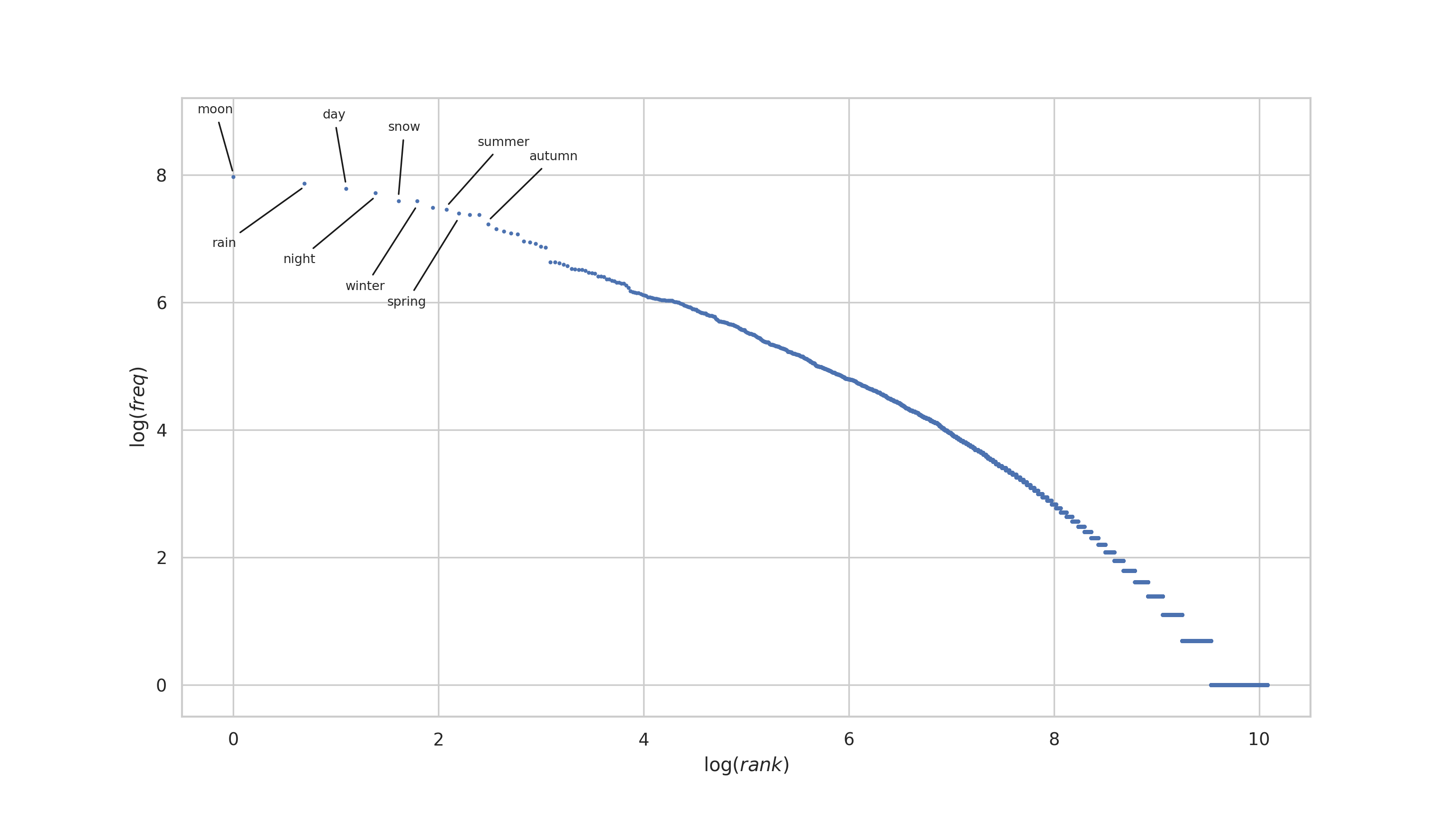

The annotated log-log plot for the haiku corpus without stopwords

So my conclusion, is that yes! haiku are a compressed form of expression, and that compression is observable by comparing the rank vs frequency plots of the haiku corpus with that of an English prose corpus (Bierce, in this case).